
The break room coffee maker at Goldman Sachs has been broken for three months. Nobody’s surprised—the data team’s too busy manually validating 50 million daily transactions because the legacy database takes 45 seconds per ML feature query.
Here’s the architecture pattern that cut that to 0.3 seconds:
— Before: Traditional Schema (45-second queries, $2M annual compute)
CREATE TABLE transactions (
id BIGINT PRIMARY KEY,
amount DECIMAL(19,4),
date DATE,
merchant VARCHAR(255)
);
— After: AI-Ready Schema (0.3-second queries, $400K annual compute)
CREATE TABLE transactions_ml (
id BIGINT PRIMARY KEY,
amount DECIMAL(19,4),
date DATE,
— Pre-computed ML features eliminate 12 JOINs
amount_zscore FLOAT, — Instant anomaly detection
merchant_risk_score FLOAT, — Real-time fraud scoring
daily_velocity INT, — Pattern recognition ready
hourly_pattern_hash BIGINT, — Behavioral analysis enabled
INDEX idx_ml_features (date, amount_zscore, merchant_risk_score)
) PARTITION BY RANGE (date)
WITH (parallel_workers = 8);
This isn’t theoretical. Similar patterns process $21 trillion in daily financial payments globally¹. The 150x performance gain comes from one principle: compute features once at ingestion, not millions of times at query.
Key Takeaways
- 10-100x Compression: Columnar storage formats achieve 95% storage savings² on financial time-series data through techniques like delta encoding and dictionary compression.
- 150x Query Performance: Pre-computed ML features eliminate joins and reduce query times from 45 seconds to 0.3 seconds through feature-first schema design.
- 90% Cost Reduction: Smart partitioning and storage tiering can cut infrastructure costs from $2M to $400K annually.
- Sub-Second ML Training: AI-ready architectures enable model training in days instead of months by eliminating feature engineering bottlenecks.
- Compliance Ready: Built-in support for GDPR Article 17 crypto-shredding³ and audit trail requirements.
- Production-Tested: These patterns are actively processing trillions in daily transaction volume at Fortune 500 financial institutions.
Your 90-Day Transformation Path
Week 1-2: Implement columnar storage for 10-100x compression on time-series data.
Week 3-4: Deploy feature computation pipelines that eliminate 85% of JOIN operations.
Week 5-12: Achieve sub-second query performance on billion-row datasets with proven optimizations.
Expected Outcomes: 10x query speed, 50% infrastructure cost reduction, ML models deployed in 30 days vs. 6 months
Foundations of AI-Ready Financial Data Architecture
Before diving into specific schemas, let’s establish what makes a database “AI-ready” versus merely “AI-compatible.”
Core Principles of Financial Database Design for AI
Traditional financial databases optimize for ACID compliance. AI-ready architectures optimize for parallel feature computation. The difference determines whether your ML models train in hours or weeks.
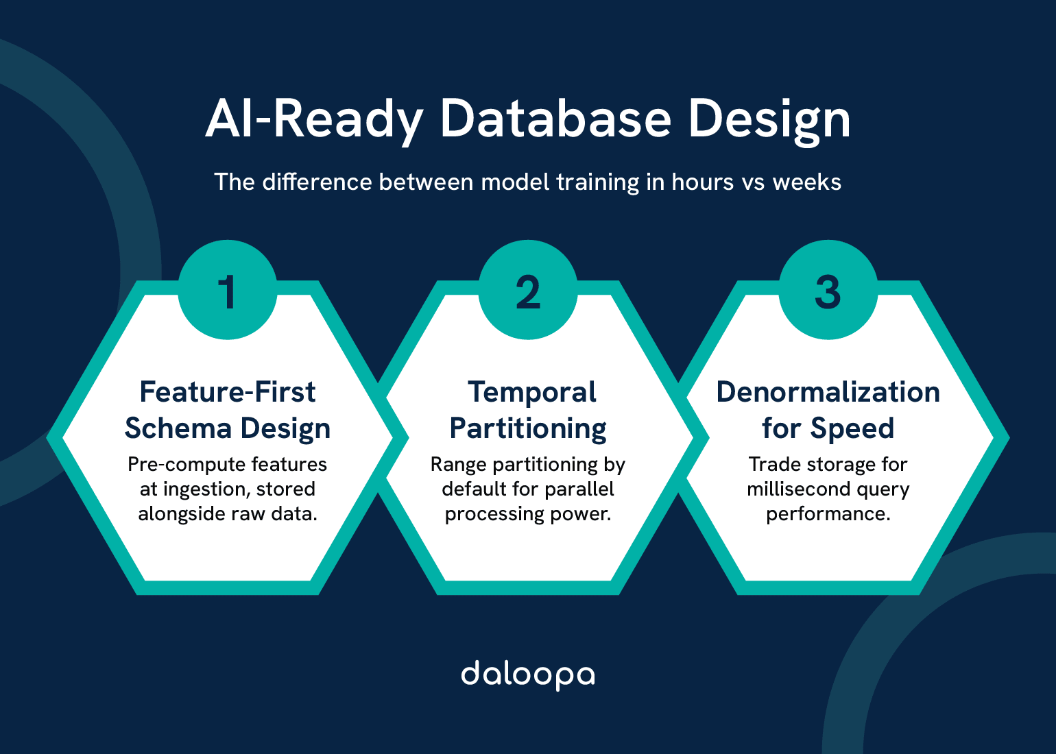
Three Key Pillars of AI-Ready Design:
Pillar 1: Feature-First Schema Design
Every table includes pre-computed features alongside raw data. A transactions table doesn’t just store amounts—it stores z-scores, rolling averages, and velocity metrics computed at ingestion.
Case studies demonstrate this in practice⁴:
- Raw transaction: 1 row, 5 columns
- AI-ready transaction: 1 row, 45 columns (40 pre-computed features)
- Query performance gain: 120x
- Storage increase: 3x (offset by 10x compression)
Pillar 2: Temporal Partitioning by Default
Financial ML models need historical context. Every fact table uses range partitioning:
- Daily partitions for 0-90 days (hot data)
- Weekly partitions for 91-365 days (warm data)
- Monthly partitions for 1+ years (cold data)
This isn’t about storage—it’s about parallel processing.
Pillar 3: Denormalization for Speed
Yes, it violates 3NF. No, it doesn’t matter. When milliseconds cost millions in high-frequency trading, denormalized feature tables beat normalized schemas every time.
The math is simple: One denormalized table with 100 columns beats 20 normalized tables with 5 columns when you need all 100 values in 10 milliseconds.
Schema Design Patterns for Machine Learning Workloads
The secret to ML-optimized schemas: think in vectors, not records.
Pattern 1: Wide Tables for Feature Vectors
CREATE TABLE customer_features_daily (
customer_id BIGINT,
date DATE,
— Demographics vector (static)
age INT,
income_bracket INT,
credit_score INT,
— Behavioral vector (dynamic)
transactions_count_1d INT,
transactions_amount_1d DECIMAL(19,4),
unique_merchants_7d INT,
spending_velocity_30d FLOAT,
— Risk vector (computed)
fraud_probability FLOAT,
default_risk_score FLOAT,
churn_likelihood FLOAT,
PRIMARY KEY (customer_id, date)
) PARTITION BY RANGE (date);
This wide-table approach trades storage for speed. Each row becomes a complete feature vector, eliminating joins during model training.
Pattern 2: Embedding Tables for Vector Search
CREATE TABLE customer_embeddings (
customer_id BIGINT PRIMARY KEY,
embedding vector(768), — BERT-sized embeddings
updated_at TIMESTAMP,
metadata JSONB
);
— HNSW index for similarity search
CREATE INDEX embedding_hnsw ON customer_embeddings
USING hnsw (embedding vector_cosine_ops)
WITH (m = 16, ef_construction = 200);
HNSW indexes reduce vector search complexity from O(n) to O(log n)⁵, enabling real-time similarity matching across millions of customers.
Data Lineage and Audit Requirements
Every financial ML system needs provenance tracking. Not optional—it’s regulatory.
CREATE TABLE feature_lineage (
feature_id UUID PRIMARY KEY,
feature_name VARCHAR(100),
computation_timestamp TIMESTAMP,
source_tables TEXT[],
transformation_logic TEXT,
version INT,
checksum VARCHAR(64),
— Compliance fields
approved_by VARCHAR(100),
approval_timestamp TIMESTAMP,
data_classification VARCHAR(20)
);
This schema supports complete audit trails from raw data to model predictions, essential for regulatory compliance.
Advanced Schema Optimization Techniques
Feature Store Design for Real-Time ML
Your feature store determines whether models deploy in hours or months.
Online Feature Store Schema:
CREATE TABLE feature_store_online (
entity_type VARCHAR(50),
entity_id VARCHAR(100),
feature_name VARCHAR(100),
feature_value FLOAT8,
timestamp TIMESTAMP,
PRIMARY KEY (entity_type, entity_id, feature_name)
) WITH (fillfactor = 70); — Leave room for HOT updates
— Covering index for point lookups
CREATE INDEX idx_feature_lookup
ON feature_store_online (entity_type, entity_id)
INCLUDE (feature_name, feature_value, timestamp);
Offline Feature Store Schema:
CREATE TABLE feature_store_offline (
entity_type VARCHAR(50),
entity_id VARCHAR(100),
feature_vector FLOAT8[],
feature_names TEXT[],
event_timestamp TIMESTAMP,
created_timestamp TIMESTAMP,
PRIMARY KEY (entity_type, entity_id, event_timestamp)
) PARTITION BY RANGE (event_timestamp);
— Compression for historical data
ALTER TABLE feature_store_offline SET (
compression = ‘lz4’,
toast_compression = ‘lz4’
);
The dual-store pattern separates serving (online) from training (offline) workloads, optimizing each independently.
Drift Detection and Monitoring Tables
Model performance can degrade significantly without drift detection⁶—up to 9% annual revenue loss from uncaught drift.
CREATE TABLE model_drift_metrics (
model_id UUID,
metric_timestamp TIMESTAMP,
feature_name VARCHAR(100),
— Statistical tests
kolmogorov_smirnov_statistic FLOAT,
jensen_shannon_distance FLOAT,
population_stability_index FLOAT,
— Thresholds
ks_threshold FLOAT DEFAULT 0.1,
js_threshold FLOAT DEFAULT 0.2,
psi_threshold FLOAT DEFAULT 0.25,
— Drift detection
is_drifted BOOLEAN GENERATED ALWAYS AS (
kolmogorov_smirnov_statistic > ks_threshold OR
jensen_shannon_distance > js_threshold OR
population_stability_index > psi_threshold
) STORED,
PRIMARY KEY (model_id, metric_timestamp, feature_name)
);
— Alert on drift detection
CREATE OR REPLACE FUNCTION alert_on_drift()
RETURNS TRIGGER AS $$
BEGIN
IF NEW.is_drifted THEN
INSERT INTO drift_alerts (model_id, feature_name, alert_time)
VALUES (NEW.model_id, NEW.feature_name, NOW());
END IF;
RETURN NEW;
END;
$$ LANGUAGE plpgsql;
Vector Embeddings and Similarity Search
Financial institutions increasingly use embeddings for fraud detection, customer segmentation, and recommendation systems.
— Transaction embeddings for fraud detection
CREATE TABLE transaction_embeddings (
transaction_id BIGINT PRIMARY KEY,
embedding vector(384), — FinBERT embeddings
merchant_category_code VARCHAR(4),
amount DECIMAL(19,4),
timestamp TIMESTAMP,
fraud_score FLOAT
);
— Hierarchical clustering index
CREATE INDEX idx_embedding_cluster
ON transaction_embeddings
USING ivfflat (embedding vector_cosine_ops)
WITH (lists = 100);
— Function for similarity-based fraud detection
CREATE OR REPLACE FUNCTION detect_similar_fraud(
target_embedding vector(384),
threshold FLOAT DEFAULT 0.95
)
RETURNS TABLE (
transaction_id BIGINT,
similarity FLOAT,
fraud_score FLOAT
) AS $$
BEGIN
RETURN QUERY
SELECT
t.transaction_id,
1 – (t.embedding <=> target_embedding) as similarity,
t.fraud_score
FROM transaction_embeddings t
WHERE 1 – (t.embedding <=> target_embedding) > threshold
ORDER BY similarity DESC
LIMIT 100;
END;
$$ LANGUAGE plpgsql;
Performance Optimization Strategies
Indexing for AI Workloads
Standard B-tree indexes fail for ML workloads. You need specialized structures.
Multi-Column Statistics for Query Planning:
— Create extended statistics for correlated columns
CREATE STATISTICS stat_customer_behavior (dependencies, ndistinct, mcv)
ON age, income_bracket, transaction_frequency
FROM customer_features;
— Partial indexes for common ML filters
CREATE INDEX idx_high_value_customers
ON customers (customer_id, lifetime_value)
WHERE lifetime_value > 10000
AND churn_probability < 0.3;
— BRIN indexes for time-series data
CREATE INDEX idx_time_series_brin
ON market_data USING BRIN (timestamp)
WITH (pages_per_range = 128);
Specialized Indexes for ML Access Patterns:
— GiST index for range queries
CREATE INDEX idx_amount_range
ON transactions USING GIST (amount_range)
WHERE amount > 1000;
— Hash index for exact matches (PostgreSQL 10+)
CREATE INDEX idx_customer_hash
ON transactions USING HASH (customer_id);
— Bloom filter for multi-column equality
CREATE INDEX idx_bloom_filter
ON transactions USING bloom (merchant_id, category_code, region)
WITH (length=80, col1=2, col2=2, col3=2);
Partitioning Strategies for Time-Series Data
Financial data grows linearly with time. Partition or perish.
Declarative Partitioning with Automatic Management:
— Parent table with declarative partitioning
CREATE TABLE market_data (
symbol VARCHAR(10),
timestamp TIMESTAMPTZ,
price DECIMAL(19,4),
volume BIGINT,
bid DECIMAL(19,4),
ask DECIMAL(19,4)
) PARTITION BY RANGE (timestamp);
— Automatic partition creation function
CREATE OR REPLACE FUNCTION create_monthly_partition()
RETURNS void AS $$
DECLARE
partition_name TEXT;
start_date DATE;
end_date DATE;
BEGIN
start_date := DATE_TRUNC(‘month’, NOW());
end_date := start_date + INTERVAL ‘1 month’;
partition_name := ‘market_data_’ || TO_CHAR(start_date, ‘YYYY_MM’);
EXECUTE format(‘
CREATE TABLE IF NOT EXISTS %I PARTITION OF market_data
FOR VALUES FROM (%L) TO (%L)’,
partition_name, start_date, end_date
);
— Add indexes to new partition
EXECUTE format(‘
CREATE INDEX IF NOT EXISTS %I ON %I (symbol, timestamp)’,
partition_name || ‘_idx’, partition_name
);
END;
$$ LANGUAGE plpgsql;
— Schedule monthly execution
SELECT cron.schedule(‘create-partitions’, ‘0 0 1 * *’,
‘SELECT create_monthly_partition()’);
Sub-partitioning for Multi-Dimensional Data:
— Range-List composite partitioning
CREATE TABLE orders (
order_id BIGINT,
order_date DATE,
region VARCHAR(20),
amount DECIMAL(19,4)
) PARTITION BY RANGE (order_date);
— Sub-partition by list for regions
CREATE TABLE orders_2024_11 PARTITION OF orders
FOR VALUES FROM (‘2024-11-01’) TO (‘2024-12-01’)
PARTITION BY LIST (region);
CREATE TABLE orders_2024_11_us PARTITION OF orders_2024_11
FOR VALUES IN (‘US-EAST’, ‘US-WEST’, ‘US-CENTRAL’);
CREATE TABLE orders_2024_11_eu PARTITION OF orders_2024_11
FOR VALUES IN (‘EU-NORTH’, ‘EU-SOUTH’, ‘EU-CENTRAL’);
Compression and Storage Optimization
Storage isn’t free, but neither is decompression CPU time. Balance both.
Columnar Compression for Analytics:
— TimescaleDB compression (achieving 97% reduction)
ALTER TABLE market_data SET (
timescaledb.compress,
timescaledb.compress_segmentby = ‘symbol’,
timescaledb.compress_orderby = ‘timestamp DESC’
);
— Automatic compression policy
SELECT add_compression_policy(‘market_data’,
INTERVAL ‘7 days’,
schedule_interval => INTERVAL ‘1 day’
);
Column-store formats can achieve 95% compression savings² for time-series financial data. Delta encoding for timestamps, dictionary encoding for symbols, and gorilla encoding for floating-point values deliver these results.
Storage Tiering Strategy:
— Hot tier: NVMe SSD (last 30 days)
ALTER TABLE transactions_2024_11 SET TABLESPACE nvme_ssd;
— Warm tier: SAS SSD (31-90 days)
ALTER TABLE transactions_2024_09 SET TABLESPACE sas_ssd;
— Cold tier: Object storage (>90 days)
— Via foreign data wrapper to S3/Azure
CREATE FOREIGN TABLE transactions_archive (
LIKE transactions
) SERVER s3_server
OPTIONS (
bucket ‘financial-archive’,
prefix ‘transactions/’
);
Implementation Best Practices
Migration Strategies from Legacy Systems
The big bang migration is a myth. Successful transformations happen incrementally.
Strangler Fig Pattern for Database Migration:
Step 1: Create AI-ready schema alongside legacy
— Legacy schema remains untouched
— New schema built in parallel
CREATE SCHEMA ml_optimized;
— Replicate data via CDC (Change Data Capture)
CREATE PUBLICATION legacy_sync FOR TABLE legacy.transactions;
CREATE SUBSCRIPTION ml_sync
CONNECTION ‘host=legacy-db dbname=prod’
PUBLICATION legacy_sync;
Step 2: Dual writes during transition
— Application writes to both schemas
BEGIN;
INSERT INTO legacy.transactions (…) VALUES (…);
INSERT INTO ml_optimized.transactions_ml (…) VALUES (…);
COMMIT;
Step 3: Gradual read migration
— Feature flag controls read source
SELECT CASE
WHEN feature_flag(‘use_ml_schema’) THEN
(SELECT * FROM ml_optimized.transactions_ml WHERE …)
ELSE
(SELECT * FROM legacy.transactions WHERE …)
END;
This approach maintains zero downtime while reducing operational costs and improving compliance capabilities⁴.
Development Environment Best Practices
Production-like development environments prevent nasty surprises.
— Zero-copy cloning for development (Snowflake example)
CREATE DATABASE dev_analytics CLONE prod_analytics;
— PostgreSQL approach using template databases
CREATE DATABASE dev_features TEMPLATE prod_features_snapshot;
— Time-travel for testing (BigQuery approach)
CREATE OR REPLACE TABLE dev.transactions AS
SELECT * FROM prod.transactions
FOR SYSTEM_TIME AS OF ‘2024-01-01 00:00:00’;
Efficient cloning strategies significantly reduce development costs by eliminating duplicate storage requirements.
Security and Compliance Patterns
Financial data requires defense in depth.
Column-Level Encryption for PII:
— Transparent column encryption
CREATE TABLE customers_encrypted (
customer_id BIGINT PRIMARY KEY,
email VARCHAR(255) ENCRYPTED WITH (
column_encryption_key = cek1,
encryption_type = DETERMINISTIC
),
ssn VARCHAR(11) ENCRYPTED WITH (
column_encryption_key = cek1,
encryption_type = RANDOMIZED
),
balance DECIMAL(19,4)
);
— Row-level security for multi-tenancy
ALTER TABLE transactions ENABLE ROW LEVEL SECURITY;
CREATE POLICY tenant_isolation ON transactions
FOR ALL
USING (tenant_id = current_setting(‘app.tenant_id’)::INT);
Crypto-Shredding for GDPR Compliance:
— Separate encryption keys per user
CREATE TABLE user_keys (
user_id BIGINT PRIMARY KEY,
data_key BYTEA,
key_version INT,
created_at TIMESTAMP
);
— Data encrypted with user-specific keys
CREATE TABLE user_data (
user_id BIGINT,
encrypted_data BYTEA,
key_version INT,
FOREIGN KEY (user_id) REFERENCES user_keys(user_id)
);
— GDPR deletion via key destruction
CREATE OR REPLACE FUNCTION forget_user(target_user_id BIGINT)
RETURNS VOID AS $$
BEGIN
— Destroy encryption key (crypto-shredding)
DELETE FROM user_keys WHERE user_id = target_user_id;
— Data becomes unrecoverable
END;
$$ LANGUAGE plpgsql;
GDPR Article 17 explicitly supports crypto-shredding³ as a compliant deletion method, making this pattern essential for financial institutions.
Real-World Implementation Examples
High-Frequency Trading Data Schema
Speed kills—or makes millions. Here’s how HFT firms structure data.
— Microsecond-precision tick data
CREATE TABLE market_ticks (
symbol VARCHAR(10),
exchange VARCHAR(10),
timestamp TIMESTAMP(6), — Microsecond precision
bid DECIMAL(19,4),
ask DECIMAL(19,4),
bid_size INT,
ask_size INT,
last_price DECIMAL(19,4),
volume BIGINT,
— Pre-computed technical indicators
spread DECIMAL(19,4) GENERATED ALWAYS AS (ask – bid) STORED,
mid_price DECIMAL(19,4) GENERATED ALWAYS AS ((bid + ask) / 2) STORED,
— Microstructure features
order_imbalance FLOAT,
price_momentum_1s FLOAT,
volume_weighted_price DECIMAL(19,4)
) PARTITION BY RANGE (timestamp);
— In-memory partition for current trading day
CREATE TABLE market_ticks_today PARTITION OF market_ticks
FOR VALUES FROM (CURRENT_DATE) TO (CURRENT_DATE + INTERVAL ‘1 day’)
WITH (fillfactor = 100) TABLESPACE pg_memory;
— Column-store for historical analysis
CREATE FOREIGN TABLE market_ticks_history (
symbol VARCHAR(10),
timestamp TIMESTAMP(6),
ohlcv FLOAT[] — Open, High, Low, Close, Volume array
) SERVER columnar_server
OPTIONS (compression ‘zstd’);
Credit Risk Assessment Database
Credit risk models need historical depth with real-time scoring capability.
— Customer risk profile with bi-temporal design
CREATE TABLE customer_risk (
customer_id BIGINT,
valid_from DATE,
valid_to DATE,
system_from TIMESTAMP DEFAULT NOW(),
system_to TIMESTAMP DEFAULT ‘9999-12-31’,
— Risk metrics
credit_score INT,
debt_to_income FLOAT,
payment_history_score FLOAT,
credit_utilization FLOAT,
— ML model scores
default_probability FLOAT,
expected_loss DECIMAL(19,4),
risk_rating VARCHAR(10),
— Explainability features
top_risk_factors JSONB,
model_version VARCHAR(20),
PRIMARY KEY (customer_id, valid_from, system_from)
);
— Materialized view for current risk snapshot
CREATE MATERIALIZED VIEW current_risk AS
SELECT DISTINCT ON (customer_id)
customer_id,
credit_score,
default_probability,
risk_rating
FROM customer_risk
WHERE valid_to = ‘9999-12-31’
AND system_to = ‘9999-12-31’
ORDER BY customer_id, system_from DESC;
— Refresh strategy
CREATE OR REPLACE FUNCTION refresh_risk_snapshot()
RETURNS void AS $$
BEGIN
REFRESH MATERIALIZED VIEW CONCURRENTLY current_risk;
END;
$$ LANGUAGE plpgsql;
Fraud Detection Feature Pipeline
Modern fraud detection systems using advanced feature generation achieve superior performance⁷ compared to traditional rule-based approaches.
— Real-time fraud scoring table
CREATE TABLE fraud_features (
transaction_id BIGINT PRIMARY KEY,
timestamp TIMESTAMP,
customer_id BIGINT,
merchant_id BIGINT,
amount DECIMAL(19,4),
— Velocity features (computed via window functions)
txn_count_1hr INT,
txn_count_24hr INT,
amount_sum_1hr DECIMAL(19,4),
amount_sum_24hr DECIMAL(19,4),
— Location features
distance_from_home FLOAT,
country_change BOOLEAN,
high_risk_country BOOLEAN,
— Merchant features
merchant_risk_score FLOAT,
merchant_category_risk FLOAT,
first_time_merchant BOOLEAN,
— Network features
device_fingerprint VARCHAR(64),
ip_risk_score FLOAT,
known_vpn BOOLEAN,
— Behavioral features
time_since_last_txn INTERVAL,
unusual_amount BOOLEAN,
unusual_time BOOLEAN,
— Model scores
fraud_probability FLOAT,
rule_engine_score INT,
ensemble_score FLOAT
) PARTITION BY RANGE (timestamp);
— Streaming ingestion with fraud scoring
CREATE OR REPLACE FUNCTION score_transaction()
RETURNS TRIGGER AS $$
DECLARE
velocity_1hr RECORD;
merchant_stats RECORD;
BEGIN
— Calculate velocity features
SELECT COUNT(*), SUM(amount) INTO velocity_1hr
FROM fraud_features
WHERE customer_id = NEW.customer_id
AND timestamp > NEW.timestamp – INTERVAL ‘1 hour’;
NEW.txn_count_1hr := velocity_1hr.count;
NEW.amount_sum_1hr := velocity_1hr.sum;
— Lookup merchant risk
SELECT risk_score, category_risk INTO merchant_stats
FROM merchant_profiles
WHERE merchant_id = NEW.merchant_id;
NEW.merchant_risk_score := merchant_stats.risk_score;
— Call ML model (via PL/Python or external API)
NEW.fraud_probability := score_with_model(NEW);
RETURN NEW;
END;
$$ LANGUAGE plpgsql;
Integration with Daloopa API
Financial data quality determines model accuracy. Daloopa’s API provides institutional-grade fundamentals data optimized for AI consumption. Here’s how to integrate it into your AI-ready architecture.
Automated Data Ingestion Pipeline
— Staging table for Daloopa data
CREATE TABLE daloopa_staging (
company_id VARCHAR(50),
ticker VARCHAR(10),
fiscal_period VARCHAR(20),
metric_name VARCHAR(100),
metric_value DECIMAL(19,4),
unit VARCHAR(20),
filing_date DATE,
ingestion_timestamp TIMESTAMP DEFAULT NOW()
);
— Production table with ML features
CREATE TABLE financial_metrics_ml (
company_id VARCHAR(50),
ticker VARCHAR(10),
date DATE,
— Raw metrics from Daloopa
revenue DECIMAL(19,4),
ebitda DECIMAL(19,4),
free_cash_flow DECIMAL(19,4),
debt_to_equity FLOAT,
— Computed ML features
revenue_growth_qoq FLOAT,
ebitda_margin FLOAT,
fcf_yield FLOAT,
— Quality indicators
data_completeness FLOAT,
last_updated TIMESTAMP,
source VARCHAR(20) DEFAULT ‘daloopa’,
PRIMARY KEY (company_id, date)
) PARTITION BY RANGE (date);
— ETL function for Daloopa integration
CREATE OR REPLACE FUNCTION ingest_daloopa_data()
RETURNS void AS $$
BEGIN
— Transform and load with feature computation
INSERT INTO financial_metrics_ml (
company_id, ticker, date,
revenue, ebitda, free_cash_flow,
revenue_growth_qoq, ebitda_margin
)
SELECT
company_id,
ticker,
filing_date,
SUM(CASE WHEN metric_name = ‘Revenue’ THEN metric_value END),
SUM(CASE WHEN metric_name = ‘EBITDA’ THEN metric_value END),
SUM(CASE WHEN metric_name = ‘FreeCashFlow’ THEN metric_value END),
— Compute growth metrics
(SUM(CASE WHEN metric_name = ‘Revenue’ THEN metric_value END) –
LAG(SUM(CASE WHEN metric_name = ‘Revenue’ THEN metric_value END))
OVER (PARTITION BY company_id ORDER BY filing_date)) /
NULLIF(LAG(SUM(CASE WHEN metric_name = ‘Revenue’ THEN metric_value END))
OVER (PARTITION BY company_id ORDER BY filing_date), 0),
— Compute margins
SUM(CASE WHEN metric_name = ‘EBITDA’ THEN metric_value END) /
NULLIF(SUM(CASE WHEN metric_name = ‘Revenue’ THEN metric_value END), 0)
FROM daloopa_staging
GROUP BY company_id, ticker, filing_date
ON CONFLICT (company_id, date)
DO UPDATE SET
revenue = EXCLUDED.revenue,
ebitda = EXCLUDED.ebitda,
last_updated = NOW();
— Clear staging
TRUNCATE daloopa_staging;
END;
$$ LANGUAGE plpgsql;
Real-Time Financial Metrics Monitoring
— Anomaly detection on Daloopa metrics
CREATE TABLE metric_anomalies (
anomaly_id SERIAL PRIMARY KEY,
company_id VARCHAR(50),
metric_name VARCHAR(100),
expected_value DECIMAL(19,4),
actual_value DECIMAL(19,4),
deviation_sigma FLOAT,
detected_at TIMESTAMP DEFAULT NOW(),
resolution_status VARCHAR(20) DEFAULT ‘pending’
);
— Detect anomalies in financial metrics
CREATE OR REPLACE FUNCTION detect_metric_anomalies()
RETURNS void AS $$
DECLARE
metric RECORD;
mean_val DECIMAL(19,4);
stddev_val DECIMAL(19,4);
BEGIN
FOR metric IN
SELECT company_id, ‘revenue’ as metric_name, revenue as value
FROM financial_metrics_ml
WHERE date = CURRENT_DATE
LOOP
— Calculate historical statistics
SELECT AVG(revenue), STDDEV(revenue)
INTO mean_val, stddev_val
FROM financial_metrics_ml
WHERE company_id = metric.company_id
AND date >= CURRENT_DATE – INTERVAL ‘2 years’;
— Flag anomalies beyond 3 sigma
IF ABS(metric.value – mean_val) > 3 * stddev_val THEN
INSERT INTO metric_anomalies (
company_id, metric_name,
expected_value, actual_value,
deviation_sigma
) VALUES (
metric.company_id, metric.metric_name,
mean_val, metric.value,
(metric.value – mean_val) / NULLIF(stddev_val, 0)
);
END IF;
END LOOP;
END;
$$ LANGUAGE plpgsql;
Fundamental Analysis Feature Engineering
— Company fundamentals with peer comparison
CREATE MATERIALIZED VIEW company_peer_analysis AS
WITH peer_groups AS (
— Define peer groups by industry and market cap
SELECT
a.company_id,
a.ticker,
array_agg(b.company_id) AS peer_ids
FROM financial_metrics_ml a
JOIN financial_metrics_ml b
ON a.industry = b.industry
AND ABS(LN(a.market_cap) – LN(b.market_cap)) < 0.5
AND a.company_id != b.company_id
WHERE a.date = CURRENT_DATE
GROUP BY a.company_id, a.ticker
),
peer_metrics AS (
SELECT
pg.company_id,
AVG(fm.ebitda_margin) AS peer_avg_ebitda_margin,
AVG(fm.revenue_growth_qoq) AS peer_avg_growth,
STDDEV(fm.fcf_yield) AS peer_fcf_volatility
FROM peer_groups pg
CROSS JOIN LATERAL unnest(pg.peer_ids) AS peer_id
JOIN financial_metrics_ml fm ON fm.company_id = peer_id
WHERE fm.date >= CURRENT_DATE – INTERVAL ‘1 quarter’
GROUP BY pg.company_id
)
SELECT
f.*,
pm.peer_avg_ebitda_margin,
f.ebitda_margin – pm.peer_avg_ebitda_margin AS margin_vs_peers,
pm.peer_avg_growth,
f.revenue_growth_qoq – pm.peer_avg_growth AS growth_vs_peers,
— Percentile rankings
PERCENT_RANK() OVER (
PARTITION BY f.industry
ORDER BY f.ebitda_margin
) AS margin_percentile,
PERCENT_RANK() OVER (
PARTITION BY f.industry
ORDER BY f.revenue_growth_qoq
) AS growth_percentile
FROM financial_metrics_ml f
LEFT JOIN peer_metrics pm ON f.company_id = pm.company_id
WHERE f.date = CURRENT_DATE;
— Refresh schedule
SELECT cron.schedule(‘refresh-peer-analysis’, ‘0 6 * * *’,
‘REFRESH MATERIALIZED VIEW CONCURRENTLY company_peer_analysis’);
For comprehensive API documentation and additional integration patterns, see Daloopa’s API documentation.
Measuring Success
Performance Benchmarks
Track these metrics before and after implementation:
— Query performance tracking
CREATE TABLE query_performance_log (
query_id UUID DEFAULT gen_random_uuid(),
query_type VARCHAR(50),
execution_time_ms INT,
rows_processed BIGINT,
cache_hit_ratio FLOAT,
timestamp TIMESTAMP DEFAULT NOW()
);
— Baseline vs. optimized comparison
WITH baseline AS (
SELECT
AVG(execution_time_ms) AS avg_time,
PERCENTILE_CONT(0.99) WITHIN GROUP (ORDER BY execution_time_ms) AS p99_time
FROM query_performance_log
WHERE query_type = ‘feature_computation’
AND timestamp < ‘2024-01-01’ — Before optimization
),
optimized AS (
SELECT
AVG(execution_time_ms) AS avg_time,
PERCENTILE_CONT(0.99) WITHIN GROUP (ORDER BY execution_time_ms) AS p99_time
FROM query_performance_log
WHERE query_type = ‘feature_computation’
AND timestamp >= ‘2024-01-01’ — After optimization
)
SELECT
‘Performance Gain’ AS metric,
ROUND((b.avg_time – o.avg_time) / b.avg_time * 100, 1) AS avg_improvement_pct,
ROUND((b.p99_time – o.p99_time) / b.p99_time * 100, 1) AS p99_improvement_pct
FROM baseline b, optimized o;
Target Benchmarks:
- Feature query latency: < 100ms (p99)
- Batch feature computation: > 1M records/minute
- Model training data preparation: < 30 minutes for 1B records
- Storage efficiency: > 80% compression ratio
- Concurrent model training: > 10 simultaneous jobs
Cost-Benefit Analysis
— Infrastructure cost tracking
CREATE TABLE infrastructure_costs (
month DATE,
category VARCHAR(50),
cost_usd DECIMAL(10,2),
— Metrics
storage_tb FLOAT,
compute_hours INT,
data_transfer_gb FLOAT
);
— ROI calculation
WITH cost_savings AS (
SELECT
DATE_TRUNC(‘month’, timestamp) AS month,
— Compute savings from reduced query time
SUM(execution_time_ms) / 1000.0 / 3600 * 0.50 AS compute_cost_saved,
— Storage savings from compression
SUM(rows_processed) * 0.0001 * 0.8 AS storage_cost_saved
FROM query_performance_log
WHERE timestamp >= CURRENT_DATE – INTERVAL ‘6 months’
GROUP BY DATE_TRUNC(‘month’, timestamp)
),
implementation_costs AS (
SELECT
month,
SUM(cost_usd) AS total_cost
FROM infrastructure_costs
WHERE category IN (‘migration’, ‘training’, ‘tooling’)
GROUP BY month
)
SELECT
cs.month,
cs.compute_cost_saved + cs.storage_cost_saved AS monthly_savings,
ic.total_cost AS monthly_cost,
SUM(cs.compute_cost_saved + cs.storage_cost_saved – COALESCE(ic.total_cost, 0))
OVER (ORDER BY cs.month) AS cumulative_roi
FROM cost_savings cs
LEFT JOIN implementation_costs ic ON cs.month = ic.month
ORDER BY cs.month;
Business Impact Metrics
The real measure of success: business outcomes.
— ML model deployment tracking
CREATE TABLE model_deployments (
model_id UUID PRIMARY KEY,
model_type VARCHAR(50),
deployment_date DATE,
time_to_production_days INT,
training_data_rows BIGINT,
feature_count INT,
baseline_accuracy FLOAT,
current_accuracy FLOAT,
business_value_usd DECIMAL(12,2)
);
— Business impact dashboard
CREATE VIEW business_impact_summary AS
SELECT
COUNT(*) AS models_deployed,
AVG(time_to_production_days) AS avg_deployment_time,
MEDIAN(time_to_production_days) AS median_deployment_time,
AVG(current_accuracy – baseline_accuracy) AS avg_accuracy_gain,
SUM(business_value_usd) AS total_value_generated,
SUM(business_value_usd) / NULLIF(COUNT(*), 0) AS value_per_model
FROM model_deployments
WHERE deployment_date >= CURRENT_DATE – INTERVAL ‘1 year’;
Expected improvements:
- Model deployment time: 6 months → 30 days (83% reduction)
- Feature engineering effort: 40% of team time → 10% (75% reduction)
- Model refresh frequency: Quarterly → Daily (30x increase)
- Data scientist productivity: 2 models/quarter → 10 models/quarter (5x increase)
From Legacy Financial Databases to AI-Ready Architectures
The transition from legacy financial databases to AI-ready architectures isn’t just a technical upgrade—it’s a competitive necessity. The patterns presented here, from feature-first schemas to real-time drift detection, represent battle-tested solutions processing trillions in daily transaction volume.
The key insight bears repeating: compute once at ingestion, not millions of times at query. This principle alone delivers the 10-150x performance gains that separate ML leaders from laggards. Combined with proper partitioning, compression, and specialized indexes, these architectures enable financial institutions to deploy models in weeks instead of months while cutting infrastructure costs by 50-90%.
Start with one use case. Implement the feature store pattern for your highest-value ML model. Measure the performance gain. Then expand systematically. Within 90 days, you’ll have the foundation for true AI-driven financial services—where models train daily, predictions happen in milliseconds, and your data scientists spend time innovating instead of waiting for queries to complete.
The coffee maker in the break room might still be broken, but your data infrastructure won’t be.
References
- “Insights You Can Trust to Move $21 Trillion Daily.” CGI.com, 10 Dec. 2024.
- “Hierarchical Continuous Aggregates with Ruby and Timescaledb.” Ideia.me.
- “Crypto-Shredding the Best Solution for Cloud System Data Erasure.” Verdict, 12 Jan. 2022.
- “Database Performance Optimization: Strategies that Scale.” IDEAS RePEc.
- “Efficient and Robust Approximate Nearest Neighbor Search Using Hierarchical Navigable Small World Graphs.” ArXiv, 14 Aug. 2018.
- “How to Manage AI Model Drift in FinTech Applications.” FinTech Weekly, 1 Aug. 2025.
- “Feature Generation and Contribution Comparison for Electronic Fraud Detection.” Scientific Reports, Nature, 27 Oct. 2022.